To precisely assess the performance of an algorithm in terms of its memory operations, we need to take into account multiple characteristics of the cache system: the number of cache layers, the memory and block sizes of each layer, the exact strategy used for cache eviction by each layer, and sometimes even the details of the memory paging mechanism.
Abstracting away from all these minor details helps a lot in the first stages of designing algorithms. Instead of calculating theoretical cache hit rates, it often makes more sense to reason about cache performance in more qualitative terms.
In this context, we can talk about the degree of cache reuse primarily in two ways:
- Temporal locality refers to the repeated access of the same data within a relatively small time period, such that the data likely remains cached between the requests.
- Spatial locality refers to the use of elements relatively close to each other in terms of their memory locations, such that they are likely fetched in the same memory block.
In other words, temporal locality is when it is likely that this same memory location will soon be requested again, while spatial locality is when it is likely that a nearby location will be requested right after.
In this section, we will do some case studies to show how these high-level concepts can help in practical optimization.
#Depth-First vs. Breadth-First
Consider a divide-and-conquer algorithm such as merge sorting. There are two approaches to implementing it:
- We can implement it recursively, or “depth-first,” the way it is normally implemented: sort the left half, sort the right half and then merge the results.
- We can implement it iteratively, or “breadth-first:” do the lowest “layer” first, looping through the entire dataset and comparing odd elements with even elements, then merge the first two elements with the second two elements, the third two elements with the fourth two elements and so on.
It seems like the second approach is more cumbersome, but faster — because recursion is always slow, right?
Generally, recursion is indeed slow, but this is not the case for this and many similar divide-and-conquer algorithms. Although the iterative approach has the advantage of only doing sequential I/O, the recursive approach has much better temporal locality: when a segment fully fits into the cache, it stays there for all lower layers of recursion, resulting in better access times later on.
In fact, since we only need to split the array $O(\log \frac{N}{M})$ times until this happens, we would only need to read $O(\frac{N}{B} \log \frac{N}{M})$ blocks in total, while in the iterative approach the entire array will be read from scratch $O(\log N)$ times no matter what. This results in the speedup of $O(\frac{\log N}{\log N - \log M})$, which may be up to an order of magnitude.
In practice, there is still some overhead associated with the recursion, and for this reason, it makes sense to use hybrid algorithms where we don’t go all the way down to the base case and instead switch to the iterative code on the lower levels of recursion.
#Dynamic Programming
Similar reasoning can be applied to the implementations of dynamic programming algorithms but leading to the reverse result. Consider the classic knapsack problem: given $N$ items with positive integer costs $c_i$, pick a subset of items with the maximum total cost that does not exceed a given constant $W$.
The way to solve it is to introduce the state $f[n, w]$, which corresponds to the maximum total cost not exceeding $w$ that can be achieved using only the first $n$ items. These values can be computed in $O(1)$ time per entry if we consider either taking or not taking the $n$-th item and using the previous states of the dynamic to make the optimal decision.
Python has a handy lru_cache decorator which can be used for implementing it with memoized recursion:
@lru_cache
def f(n, w):
    # check if we have no items to choose
    if n == 0:
        return 0

    # check if we can't pick the last item (note zero-based indexing)
    if c[n - 1] > w:
        return f(n - 1, w)

    # otherwise, we can either pick the last item or not
    return max(f(n - 1, w), c[n - 1] + f(n - 1, w - c[n - 1]))
When computing $f[N, W]$, the recursion may visit up to $O(N \cdot W)$ different states, which is asymptotically efficient, but rather slow in reality. Even after nullifying the overhead of Python recursion and all the hash table queries required for the LRU cache to work, it would still be slow because it does random I/O throughout most of the execution.
What we can do instead is to create a two-dimensional array for the dynamic and replace the recursion with a nice nested loop like this:
int f[N + 1][W + 1] = {0}; // this zero-fills the array

for (int n = 1; n <= N; n++)
    for (int w = 0; w <= W; w++)
        f[n][w] = c[n - 1] > w ?
                  f[n - 1][w] :
                  max(f[n - 1][k], c[n - 1] + f[n - 1][w - c[n - 1]]);
Notice that we are only using the previous layer of the dynamic to calculate the next one. This means that if we can store one layer in the cache, we would only need to write $O(\frac{N \cdot W}{B})$ blocks in external memory.
Moreover, if we only need the answer, we don’t actually have to store the whole 2d array but only the last layer. This lets us use just $O(W)$ memory by maintaining a single array of $W$ values. To simplify the code, we can slightly change the dynamic to store a binary value: whether it is possible to get the sum of exactly $w$ using the items that we have already considered. This dynamic is even faster to compute:
bool f[W + 1] = {0};
f[0] = 1;
for (int n = 0; n < N; n++)
    for (int x = W - c[n]; x >= 0; x--)
        f[x + c[n]] |= f[x];
As a side note, now that it only uses simple bitwise operations, it can be optimized further by using a bitset:
std::bitset<W + 1> b;
b[0] = 1;
for (int n = 0; n < N; n++)
    b |= b << c[n];
Surprisingly, there is still some room for improvement, and we will come back to this problem later.
#Sparse Table
Sparse table is a static data structure that is often used for solving the static RMQ problem and computing any similar idempotent range reductions in general. It can be formally defined as a two-dimensional array of size $\log n \times n$:
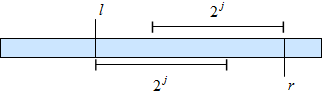
$$ t[k][i] = \min \{ a_i, a_{i+1}, \ldots, a_{i+2^k-1} \} $$In plain English: we store the minimum on each segment whose length is a power of two.
Such array can be used for calculating minima on arbitrary segments in constant time because for each segment we can always find two possibly overlapping segments whose sizes are the same power of two, the union of which gives the whole segment.
This means that we can just take the minimum of these two precomputed minimums as the answer:
int rmq(int l, int r) { // half-interval [l; r)
    int t = __lg(r - l);
    return min(mn[t][l], mn[t][r - (1 << t)]);
}
The __lg function is an intrinsic available in GCC that calculates the binary logarithm of a number rounded down. Internally it uses the clz (“count leading zeros”) instruction and subtracts this count from 32 (in case of a 32-bit integer), and thus takes just a few cycles.
The reason why I bring it up in this article is that there are multiple alternative ways it can be built, with different efficiencies in terms of memory operations. In general, a sparse table can be built in $O(n \log n)$ time in dynamic programming fashion by iterating in the order of increasing $i$ or $k$ and applying the following identity:
$$ t[k][i] = \min(t[k-1][i], t[k-1][i+2^{k-1}]) $$Now, there are two design choices to make: whether the log-size $k$ should be the first or the second dimension, and whether to iterate over $k$ and then $i$ or the other way around. This means that there are $2×2=4$ ways to build it, and here is the optimal one:
int mn[logn][maxn];

memcpy(mn[0], a, sizeof a);

for (int l = 0; l < logn - 1; l++)
    for (int i = 0; i + (2 << l) <= n; i++)
        mn[l + 1][i] = min(mn[l][i], mn[l][i + (1 << l)]);
This is the only combination of the memory layout and the iteration order that results in beautiful linear passes that work ~3x faster. As an exercise, consider the other three variants and think about why they are slower.
#Array-of-Structs vs. Struct-of-Arrays
Suppose that you want to implement a binary tree and store its fields in separate arrays like this:
int left_child[maxn], right_child[maxn], key[maxn], size[maxn];
Such memory layout, when we store each field separately from others, is called struct-of-arrays (SoA). In most cases, when implementing tree operations, you access a node and then shortly after all or most of its internal data. If these fields are stored separately, this would mean that they are also located in different memory blocks. If some of the requested fields happen to be are cached while the others are not, you would still have to wait for the slowest of them to be fetched.
In contrast, if it was instead stored as an array-of-structs (AoS), you would need ~4 times fewer block reads as all the data of a node is stored in the same block and fetched at once:
struct Node {
    int left_child, right_child, key, size;
};

Node t[maxn];
The AoS layout is usually preferred for data structures, but SoA still has good uses: while it is worse for searching, it is much better for linear scanning.
This difference in design is important in data processing applications. For example, databases can be either row- or column-oriented (also called columnar):
- Row-oriented storage formats are used when you need to search for a limited number of objects in a large dataset and/or fetch all or most of their fields. Examples: PostgreSQL, MongoDB.
- Columnar storage formats are used for big data processing and analytics, where you need to scan through everything anyway to calculate certain statistics. Examples: ClickHouse, Hbase.
Columnar formats have the additional advantage that you can only read the fields that you need, as different fields are stored in separate external memory regions.