If you ever opened a computer science textbook, it probably introduced computational complexity somewhere in the very beginning. Simply put, it is the total count of elementary operations (additions, multiplications, reads, writes…) that are executed during a computation, optionally weighted by their costs.
Complexity is an old concept. It was systematically formulated in the early 1960s, and since then it has been universally used as the cost function for designing algorithms. The reason this model was so quickly adopted is that it was a good approximation of how computers worked at the time.
Classical Complexity Theory
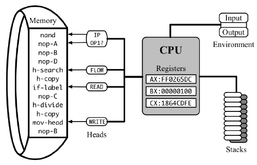
The “elementary operations” of a CPU are called instructions, and their “costs” are called latencies. Instructions are stored in memory and executed one by one by the processor, which has some internal state stored in a number of registers. One of these registers is the instruction pointer, which indicates the address of the next instruction to read and execute. Each instruction changes the state of the processor in a certain way (including moving the instruction pointer), possibly modifies the main memory, and takes a different number of CPU cycles to complete before the next one can be started.
To estimate the real running time of a program, you need to sum all latencies for its executed instructions and divide it by the clock frequency, that is, the number of cycles a particular CPU does per second.
The clock frequency is a volatile and often unknown variable that depends on the CPU model, operating system settings, current microchip temperature, power usage of other components, and quite a few other things. In contrast, instruction latencies are static and even somewhat consistent across different CPUs when expressed in clock cycles, so counting them instead is much more useful for analytical purposes.
For example, the by-definition matrix multiplication algorithm requires the total of $n^2 \cdot (n + n - 1)$ arithmetic operations: specifically, $n^3$ multiplications and $n^2 \cdot (n - 1)$ additions. If we look up the latencies for these instructions (in special documents called instruction tables, like this one), we can find that, e.g., multiplication takes 3 cycles, while addition takes 1, so we need a total of $3 \cdot n^3 + n^2 \cdot (n - 1) = 4 \cdot n^3 - n^2$ clock cycles for the entire computation (bluntly ignoring everything else that needs to be done to “feed” these instructions with the right data).
Similar to how the sum of instruction latencies can be used as a clock-independent proxy for total execution time, computational complexity can be used to quantify the intrinsic time requirements of an abstract algorithm, without relying on the choice of a specific computer.
Asymptotic Complexity
The idea to express execution time as a function of input size seems obvious now, but it wasn’t so in the 1960s. Back then, typical computers cost millions of dollars, were so large that they required a separate room, and had clock rates measured in kilohertz. They were used for practical tasks at hand, like predicting the weather, sending rockets into space, or figuring out how far a Soviet nuclear missile can fly from the coast of Cuba — all of which are finite-length problems. Engineers of that era were mainly concerned with how to multiply $3 \times 3$ matrices rather than $n \times n$ ones.
What caused the shift was the acquired confidence among computer scientists that computers will continue to become faster — and indeed they have. Over time, people stopped counting execution time, then stopped counting cycles, and then even stopped counting operations exactly, replacing it with an estimate that, on sufficiently large inputs, is only off by no more than a constant factor. With asymptotic complexity, verbose “$4 \cdot n^3 - n^2$ operations” turns into plain “$\Theta(n^3)$,” hiding the initial costs of individual operations in the “Big O,” along with all the other intricacies of the hardware.
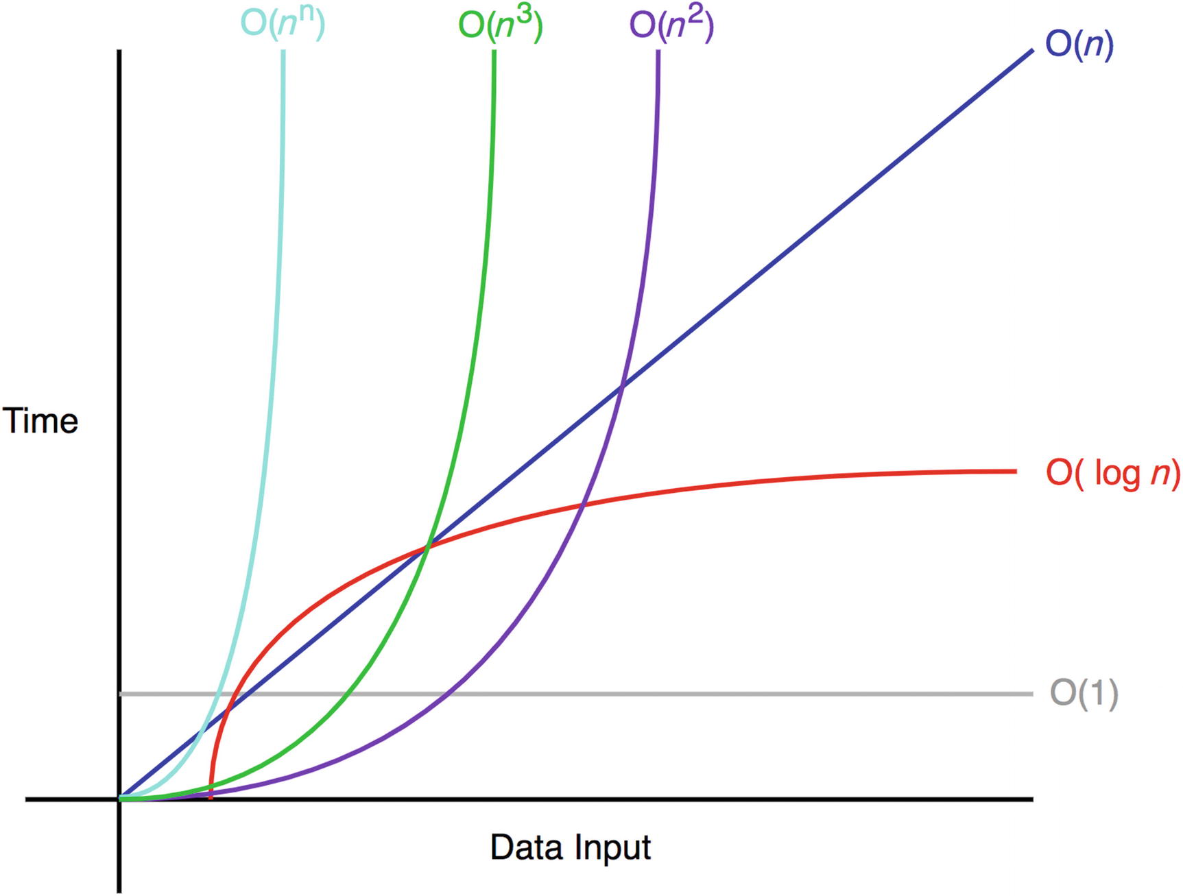
The reason we use asymptotic complexity is that it provides simplicity while still being just precise enough to yield useful results about relative algorithm performance on large datasets. Under the promise that computers will eventually become fast enough to handle any sufficiently large input in a reasonable amount of time, asymptotically faster algorithms will always be faster in real-time too, regardless of the hidden constant.
But this promise turned out to be not true — at least not in terms of clock speeds and instruction latencies — and in this chapter, we will try to explain why and how to deal with it.