Static B-Trees

This section is a follow-up to the previous one, where we optimized binary search by the means of removing branching and improving the memory layout. Here, we will also be searching in sorted arrays, but this time we are not limited to fetching and comparing only one element at a time.

In this section, we generalize the techniques we developed for binary search to static B-trees and accelerate them further using SIMD instructions. In particular, we develop two new implicit data structures:

• The first is based on the memory layout of a B-tree, and, depending on the array size, it is up to 8x faster than std::lower_bound while using the same space as the array and only requiring a permutation of its elements.
• The second is based on the memory layout of a B+ tree, and it is up to 15x faster than std::lower_bound while using just 6-7% more memory — or 6-7% of the memory if we can keep the original sorted array.

To distinguish them from B-trees — the structures with pointers, hundreds to thousands of keys per node, and empty spaces in them — we will use the names S-tree and S+ tree respectively to refer to these particular memory layouts¹.

To the best of my knowledge, this is a significant improvement over the existing approaches. As before, we are using Clang 10 targeting a Zen 2 CPU, but the performance improvements should approximately transfer to most other platforms, including Arm-based chips. Use this single-source benchmark of the final implementation if you want to test it on your machine.

This is a long article, and since it also serves as a textbook case study, we will improve the algorithm incrementally for pedagogical goals. If you are already an expert and feel comfortable reading intrinsic-heavy code with little to no context, you can jump straight to the final implementation.

#B-Tree Layout

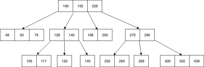
B-trees generalize the concept of binary search trees by allowing nodes to have more than two children. Instead of a single key, a node of a B-tree of order $k$ can contain up to $B = (k - 1)$ keys stored in sorted order and up to $k$ pointers to child nodes. Each child $i$ satisfies the property that all keys in its subtree are between keys $(i - 1)$ and $i$ of the parent node (if they exist).

The main advantage of this approach is that it reduces the tree height by $\frac{\log_2 n}{\log_k n} = \frac{\log k}{\log 2} = \log_2 k$ times, while fetching each node still takes roughly the same time — as long it fits into a single memory block.

B-trees were primarily developed for the purpose of managing on-disk databases, where the latency of randomly fetching a single byte is comparable with the time it takes to read the next 1MB of data sequentially. For our use case, we will be using the block size of $B = 16$ elements — or $64$ bytes, the size of the cache line — which makes the tree height and the total number of cache line fetches per query $\log_2 17 \approx 4$ times smaller compared to the binary search.

#Implicit B-Tree

Storing and fetching pointers in a B-tree node wastes precious cache space and decreases performance, but they are essential for changing the tree structure on inserts and deletions. But when there are no updates and the structure of a tree is static, we can get rid of the pointers, which makes the structure implicit.

One of the ways to achieve this is by generalizing the Eytzinger numeration to $(B + 1)$-ary trees:

• The root node is numbered $0$.
• Node $k$ has $(B + 1)$ child nodes numbered $\{k \cdot (B + 1) + i + 1\}$ for $i \in [0, B]$.

This way, we can only use $O(1)$ additional memory by allocating one large two-dimensional array of keys and relying on index arithmetic to locate children nodes in the tree:

const int B = 16;

int nblocks = (n + B - 1) / B;
int btree[nblocks][B];

int go(int k, int i) { return k * (B + 1) + i + 1; }

This numeration automatically makes the B-tree complete or almost complete with the height of $\Theta(\log_{B + 1} n)$. If the length of the initial array is not a multiple of $B$, the last block is padded with the largest value of its data type.

#Construction

We can construct the B-tree similar to how we constructed the Eytzinger array — by traversing the search tree:

void build(int k = 0) {
    static int t = 0;
    if (k < nblocks) {
        for (int i = 0; i < B; i++) {
            build(go(k, i));
            btree[k][i] = (t < n ? a[t++] : INT_MAX);
        }
        build(go(k, B));
    }
}

It is correct because each value of the initial array will be copied to a unique position in the resulting array, and the tree height is $\Theta(\log_{B+1} n)$ because $k$ is multiplied by $(B + 1)$ each time we descend into a child node.

Note that this numeration causes a slight imbalance: left-er children may have larger subtrees, although this is only true for $O(\log_{B+1} n)$ parent nodes.

#Searches

To find the lower bound, we need to fetch the $B$ keys in a node, find the first key $a_i$ not less than $x$, descend to the $i$-th child — and continue until we reach a leaf node. There is some variability in how to find that first key. For example, we could do a tiny internal binary search that makes $O(\log B)$ iterations, or maybe just compare each key sequentially in $O(B)$ time until we find the local lower bound, hopefully exiting from the loop a bit early.

But we are not going to do that — because we can use SIMD. It doesn’t work well with branching, so essentially what we want to do is to compare against all $B$ elements regardless, compute a bitmask out of these comparisons, and then use the ffs instruction to find the bit corresponding to the first non-lesser element:

int mask = (1 << B);

for (int i = 0; i < B; i++)
    mask |= (btree[k][i] >= x) << i;

int i = __builtin_ffs(mask) - 1;
// now i is the number of the correct child node

Unfortunately, the compilers are not smart enough to auto-vectorize this code yet, so we have to optimize it manually. In AVX2, we can load 8 elements, compare them against the search key, producing a vector mask, and then extract the scalar mask from it with movemask. Here is a minimized illustrated example of what we want to do:

       y = 4        17       65       103     
       x = 42       42       42       42      
   y ≥ x = 00000000 00000000 11111111 11111111
           ├┬┬┬─────┴────────┴────────┘       
movemask = 0011                               
           ┌─┘                                
     ffs = 3                                  

Since we are limited to processing 8 elements at a time (half our block / cache line size), we have to split the elements into two groups and then combine the two 8-bit masks. To do this, it will be slightly easier to swap the condition for x > y and compute the inverted mask instead:

typedef __m256i reg;

int cmp(reg x_vec, int* y_ptr) {
    reg y_vec = _mm256_load_si256((reg*) y_ptr); // load 8 sorted elements
    reg mask = _mm256_cmpgt_epi32(x_vec, y_vec); // compare against the key
    return _mm256_movemask_ps((__m256) mask);    // extract the 8-bit mask
}

Now, to process the entire block, we need to call it twice and combine the masks:

int mask = ~(
    cmp(x, &btree[k][0]) +
    (cmp(x, &btree[k][8]) << 8)
);

To descend down the tree, we use ffs on that mask to get the correct child number and just call the go function we defined earlier:

int i = __builtin_ffs(mask) - 1;
k = go(k, i);

To actually return the result in the end, we’d want to just fetch btree[k][i] in the last node we visited, but the problem is that sometimes the local lower bound doesn’t exist ($i \ge B$) because $x$ happens to be greater than all the keys in the node. We could, in theory, do the same thing we did for the Eytzinger binary search and restore the correct element after we calculate the last index, but we don’t have a nice bit trick this time and have to do a lot of divisions by 17 to compute it, which will be slow and almost certainly not worth it.

Instead, we can just remember and return the last local lower bound we encountered when we descended the tree:

int lower_bound(int _x) {
    int k = 0, res = INT_MAX;
    reg x = _mm256_set1_epi32(_x);
    while (k < nblocks) {
        int mask = ~(
            cmp(x, &btree[k][0]) +
            (cmp(x, &btree[k][8]) << 8)
        );
        int i = __builtin_ffs(mask) - 1;
        if (i < B)
            res = btree[k][i];
        k = go(k, i);
    }
    return res;
}

This implementation outperforms all previous binary search implementations, and by a huge margin:

This is very good — but we can optimize it even further.

#Optimization

Before everything else, let’s allocate the memory for the array on a hugepage:

const int P = 1 << 21;                        // page size in bytes (2MB)
const int T = (64 * nblocks + P - 1) / P * P; // can only allocate whole number of pages
btree = (int(*)[16]) std::aligned_alloc(P, T);
madvise(btree, T, MADV_HUGEPAGE);

This slightly improves the performance on larger array sizes:

Ideally, we’d also need to enable hugepages for all previous implementations to make the comparison fair, but it doesn’t matter that much because they all have some form of prefetching that alleviates this problem.

With that settled, let’s begin real optimization. First of all, we’d want to use compile-time constants instead of variables as much as possible because it lets the compiler embed them in the machine code, unroll loops, optimize arithmetic, and do all sorts of other nice stuff for us for free. Specifically, we want to know the tree height in advance:

constexpr int height(int n) {
    // grow the tree until its size exceeds n elements
    int s = 0, // total size so far
        l = B, // size of the next layer
        h = 0; // height so far
    while (s + l - B < n) {
        s += l;
        l *= (B + 1);
        h++;
    }
    return h;
}

const int H = height(N);

Next, we can find the local lower bound in nodes faster. Instead of calculating it separately for two 8-element blocks and merging two 8-bit masks, we combine the vector masks using the packs instruction and readily extract it using movemask just once:

unsigned rank(reg x, int* y) {
    reg a = _mm256_load_si256((reg*) y);
    reg b = _mm256_load_si256((reg*) (y + 8));

    reg ca = _mm256_cmpgt_epi32(a, x);
    reg cb = _mm256_cmpgt_epi32(b, x);

    reg c = _mm256_packs_epi32(ca, cb);
    int mask = _mm256_movemask_epi8(c);

    // we need to divide the result by two because we call movemask_epi8 on 16-bit masks:
    return __tzcnt_u32(mask) >> 1;
}

This instruction converts 32-bit integers stored in two registers to 16-bit integers stored in one register — in our case, effectively joining the vector masks into one. Note that we’ve swapped the order of comparison — this lets us not invert the mask in the end, but we have to subtract² one from the search key once in the beginning to make it correct (otherwise, it works as upper_bound).

The problem is, it does this weird interleaving where the result is written in the a1 b1 a2 b2 order instead of a1 a2 b1 b2 that we want — many AVX2 instructions tend to do that. To correct this, we need to permute the resulting vector, but instead of doing it during the query time, we can just permute every node during preprocessing:

void permute(int *node) {
    const reg perm = _mm256_setr_epi32(4, 5, 6, 7, 0, 1, 2, 3);
    reg* middle = (reg*) (node + 4);
    reg x = _mm256_loadu_si256(middle);
    x = _mm256_permutevar8x32_epi32(x, perm);
    _mm256_storeu_si256(middle, x);
}

Now we just call permute(&btree[k]) right after we are done building the node. There are probably faster ways to swap the middle elements, but we will leave it here as the preprocessing time is not that important for now.

This new SIMD routine is significantly faster because the extra movemask is slow, and also blending the two masks takes quite a few instructions. Unfortunately, we now can’t just do the res = btree[k][i] update anymore because the elements are permuted. We can solve this problem with some bit-level trickery in terms of i, but indexing a small lookup table turns out to be faster and also doesn’t require a new branch:

const int translate[17] = {
    0, 1, 2, 3,
    8, 9, 10, 11,
    4, 5, 6, 7,
    12, 13, 14, 15,
    0
};

void update(int &res, int* node, unsigned i) {
    int val = node[translate[i]];
    res = (i < B ? val : res);
}

This update procedure takes some time, but it’s not on the critical path between the iterations, so it doesn’t affect the actual performance that much.

Stitching it all together (and leaving out some other minor optimizations):

int lower_bound(int _x) {
    int k = 0, res = INT_MAX;
    reg x = _mm256_set1_epi32(_x - 1);
    for (int h = 0; h < H - 1; h++) {
        unsigned i = rank(x, &btree[k]);
        update(res, &btree[k], i);
        k = go(k, i);
    }
    // the last branch:
    if (k < nblocks) {
        unsigned i = rank(x, btree[k]);
        update(res, &btree[k], i);
    }
    return res;
}

All this work saved us 15-20% or so:

It doesn’t feel very satisfying so far, but we will reuse these optimization ideas later.

There are two main problems with the current implementation:

• The update procedure is quite costly, especially considering that it is very likely going to be useless: 16 out of 17 times, we can just fetch the result from the last block.
• We do a non-constant number of iterations, causing branch prediction problems similar to how it did for the Eytzinger binary search; you can also see it on the graph this time, but the latency bumps have a period of $2^4$.

To address these problems, we need to change the layout a little bit.

#B+ Tree Layout

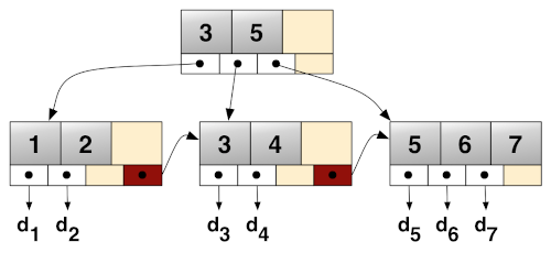
Most of the time, when people talk about B-trees, they really mean B+ trees, which is a modification that distinguishes between the two types of nodes:

• Internal nodes store up to $B$ keys and $(B + 1)$ pointers to child nodes. The key number $i$ is always equal to the smallest key in the subtree of the $(i + 1)$-th child node.
• Data nodes or leaves store up to $B$ keys, the pointer to the next leaf node, and, optionally, an associated value for each key — if the structure is used as a key-value map.

The advantages of this approach include faster search time (as the internal nodes only store keys) and the ability to quickly iterate over a range of entries (by following next leaf node pointers), but this comes at the cost of some memory overhead: we have to store copies of keys in the internal nodes.

Back to our use case, this layout can help us solve our two problems:

• Either the last node we descend into has the local lower bound, or it is the first key of the next leaf node, so we don’t need to call update on each iteration.
• The depth of all leaves is constant because B+ trees grow at the root and not at the leaves, which removes the need for branching.

The disadvantage is that this layout is not succinct: we need some additional memory to store the internal nodes — about $\frac{1}{16}$-th of the original array size, to be exact — but the performance improvement will be more than worth it.

#Implicit B+ Tree

To be more explicit with pointer arithmetic, we will store the entire tree in a single one-dimensional array. To minimize index computations during run time, we will store each layer sequentially in this array and use compile time computed offsets to address them: the keys of the node number k on layer h start with btree[offset(h) + k * B], and its i-th child will at btree[offset(h - 1) + (k * (B + 1) + i) * B].

To implement all that, we need slightly more constexpr functions:

// number of B-element blocks in a layer with n keys
constexpr int blocks(int n) {
    return (n + B - 1) / B;
}

// number of keys on the layer previous to one with n keys
constexpr int prev_keys(int n) {
    return (blocks(n) + B) / (B + 1) * B;
}

// height of a balanced n-key B+ tree
constexpr int height(int n) {
    return (n <= B ? 1 : height(prev_keys(n)) + 1);
}

// where the layer h starts (layer 0 is the largest)
constexpr int offset(int h) {
    int k = 0, n = N;
    while (h--) {
        k += blocks(n) * B;
        n = prev_keys(n);
    }
    return k;
}

const int H = height(N);
const int S = offset(H); // the tree size is the offset of the (non-existent) layer H

int *btree; // the tree itself is stored in a single hugepage-aligned array of size S

Note that we store the layers in reverse order, but the nodes within a layer and data in them are still left-to-right, and also the layers are numbered bottom-up: the leaves form the zeroth layer, and the root is the layer H - 1. These are just arbitrary decisions — it is just slightly easier to implement in code.

#Construction

To construct the tree from a sorted array a, we first need to copy it into the zeroth layer and pad it with infinities:

memcpy(btree, a, 4 * N);

for (int i = N; i < S; i++)
    btree[i] = INT_MAX;

Now we build the internal nodes, layer by layer. For each key, we need to descend to the right of it in, always go left until we reach a leaf node, and then take its first key — it will be the smallest on the subtree:

for (int h = 1; h < H; h++) {
    for (int i = 0; i < offset(h + 1) - offset(h); i++) {
        // i = k * B + j
        int k = i / B,
            j = i - k * B;
        k = k * (B + 1) + j + 1; // compare to the right of the key
        // and then always to the left
        for (int l = 0; l < h - 1; l++)
            k *= (B + 1);
        // pad the rest with infinities if the key doesn't exist 
        btree[offset(h) + i] = (k * B < N ? btree[k * B] : INT_MAX);
    }
}

And just the finishing touch — we need to permute keys in internal nodes to search them faster:

for (int i = offset(1); i < S; i += B)
    permute(btree + i);

We start from offset(1), and we specifically don’t permute leaf nodes and leave the array in the original sorted order. The motivation is that we’d need to do this complex index translation we do in update if the keys were permuted, and it is on the critical path when this is the last operation. So, just for this layer, we switch to the original mask-blending local lower bound procedure.

#Searching

The search procedure becomes simpler than for the B-tree layout: we don’t need to do update and only execute a fixed number of iterations — although the last one with some special treatment:

int lower_bound(int _x) {
    unsigned k = 0; // we assume k already multiplied by B to optimize pointer arithmetic
    reg x = _mm256_set1_epi32(_x - 1);
    for (int h = H - 1; h > 0; h--) {
        unsigned i = permuted_rank(x, btree + offset(h) + k);
        k = k * (B + 1) + i * B;
    }
    unsigned i = direct_rank(x, btree + k);
    return btree[k + i];
}

Switching to the B+ layout more than paid off: the S+ tree is 1.5-3x faster compared to the optimized S-tree:

The spikes at the high end of the graph are caused by the L1 TLB not being large enough: it has 64 entries, so it can handle at most 64 × 2 = 128MB of data, which is exactly what is required for storing 2^25 integers. The S+ tree hits this limit slightly sooner because of the ~7% memory overhead.

#Comparison with std::lower_bound

We’ve come a long way from binary search:

On these scales, it makes more sense to look at the relative speedup:

The cliffs at the beginning of the graph are because the running time of std::lower_bound grows smoothly with the array size, while for an S+ tree, it is locally flat and increases in discrete steps when a new layer needs to be added.

One important asterisk we haven’t discussed is that what we are measuring is not real latency, but the reciprocal throughput — the total time it takes to execute a lot of queries divided by the number of queries:

clock_t start = clock();

for (int i = 0; i < m; i++)
    checksum ^= lower_bound(q[i]);

float seconds = float(clock() - start) / CLOCKS_PER_SEC;
printf("%.2f ns per query\n", 1e9 * seconds / m);

To measure actual latency, we need to introduce a dependency between the loop iterations so that the next query can’t start before the previous one finishes:

int last = 0;

for (int i = 0; i < m; i++) {
    last = lower_bound(q[i] ^ last);
    checksum ^= last;
}

In terms of real latency, the speedup is not that impressive:

A lot of the performance boost of the S+ tree comes from removing branching and minimizing memory requests, which allows overlapping the execution of more adjacent queries — apparently, around three on average.

Although nobody except maybe the HFT people cares about real latency, and everybody actually measures throughput even when using the word “latency,” this nuance is still something to take into account when predicting the possible speedup in user applications.

#Modifications and Further Optimizations

To minimize the number of memory accesses during a query, we can increase the block size. To find the local lower bound in a 32-element node (spanning two cache lines and four AVX2 registers), we can use a similar trick that uses two packs_epi32 and one packs_epi16 to combine masks.

We can also try to use the cache more efficiently by controlling where each tree layer is stored in the cache hierarchy. We can do that by prefetching nodes to a specific level and using non-temporal reads during queries.

I implemented two versions of these optimizations: the one with a block size of 32 and the one where the last read is non-temporal. They don’t improve the throughput:

…but they do make the latency lower:

Ideas that I have not yet managed to implement but consider highly perspective are:

• Make the block size non-uniform. The motivation is that the slowdown from having one 32-element layer is less than from having two separate layers. Also, the root is often not full, so perhaps sometimes it should have only 8 keys or even just one key. Picking the optimal layer configuration for a given array size should remove the spikes from the relative speedup graph and make it look more like its upper envelope.

  I know how to do it with code generation, but I went for a generic solution and tried to implement it with the facilities of modern C++, but the compiler can’t produce optimal code this way.

• Group nodes with one or two generations of its descendants (~300 nodes / ~5k keys) so that they are close in memory — in the spirit of what FAST calls hierarchical blocking. This reduces the severity of TLB misses and also may improve the latency as the memory controller may choose to keep the RAM row buffer open, anticipating local reads.

• Optionally use prefetching on some specific layers. Aside from to the $\frac{1}{17}$-th chance of it fetching the node we need, the hardware prefetcher may also get some of its neighbors for us if the data bus is not busy. It also has the same TLB and row buffer effects as with blocking.

Other possible minor optimizations include:

• Permuting the nodes of the last layer as well — if we only need the index and not the value.
• Reversing the order in which the layers are stored to left-to-right so that the first few layers are on the same page.
• Rewriting the whole thing in assembly, as the compiler seems to struggle with pointer arithmetic.
• Using blending instead of packs: you can odd-even shuffle node keys ([1 3 5 7] [2 4 6 8]), compare against the search key, and then blend the low 16 bits of the first register mask with the high 16 bits of the second. Blending is slightly faster on many architectures, and it may also help to alternate between packing and blending as they use different subsets of ports. (Thanks to Const-me from HackerNews for suggesting it.)
• Using popcount instead of tzcnt: the index i is equal to the number of keys less than x, so we can compare x against all keys, combine the vector mask any way we want, call maskmov, and then calculate the number of set bits with popcnt. This removes the need to store the keys in any particular order, which lets us skip the permutation step and also use this procedure on the last layer as well.
• Defining the key $i$ as the maximum key in the subtree of child $i$ instead of the minimum key in the subtree of child $(i + 1)$. The correctness doesn’t change, but this guarantees that the result will be stored in the last node we access (and not in the first element of the next neighbor node), which lets us fetch slightly fewer cache lines.

Note that the current implementation is specific to AVX2 and may require some non-trivial changes to adapt to other platforms. It would be interesting to port it for Intel CPUs with AVX-512 and Arm CPUs with 128-bit NEON, which may require some trickery to work.

With these optimizations implemented, I wouldn’t be surprised to see another 10-30% improvement and over 10x speedup over std::lower_bound on large arrays for some platforms.

#As a Dynamic Tree

The comparison is even more favorable against std::set and other pointer-based trees. In our benchmark, we add the same elements (without measuring the time it takes to add them) and use the same lower bound queries, and the S+ tree is up to 30x faster:

This suggests that we can probably use this approach to also improve on dynamic search trees by a large margin.

To validate this hypothesis, I added an array of 17 indices for each node that point to where their children should be and used this array to descend the tree instead of the usual implicit numbering. This array is separate from the tree, not aligned, and isn’t even on a hugepage — the only optimization we do is prefetch the first and the last pointer of a node.

I also added B-tree from Abseil to the comparison, which is the only widely-used B-tree implementation I know of. It performs just slightly better than std::lower_bound, while the S+ tree with pointers is ~15x faster for large arrays:

Of course, this comparison is not fair, as implementing a dynamic search tree is a more high-dimensional problem.

We’d also need to implement the update operation, which will not be that efficient, and for which we’d need to sacrifice the fanout factor. But it still seems possible to implement a 10-20x faster std::set and a 3-5x faster absl::btree_set, depending on how you define “faster” — and this is one of the things we’ll attempt to do next.

#Acknowledgements

This StackOverflow answer by Cory Nelson is where I took the permuted 16-element search trick from.